41 add data labels excel 2013

How to Add Total Data Labels to the Excel Stacked Bar Chart Step 4: Right click your new line chart and select "Add Data Labels" Step 5: Right click your new data labels and format them so that their label position is "Above"; also make the labels bold and increase the font size. Step 6: Right click the line, select "Format Data Series"; in the Line Color menu, select "No line" Step 7 ... How to Create Address Labels from Excel on PC or Mac menu, select All Apps, open Microsoft Office, then click Microsoft Excel. If you have a Mac, open the Launchpad, then click Microsoft Excel. It may be in a folder called Microsoft Office. 2. Enter field names for each column on the first row. The first row in the sheet must contain header for each type of data.

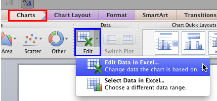
support.microsoft.com › en-us › officeMail merge using an Excel spreadsheet - support.microsoft.com Connect to your data source. For more info, see Data sources you can use for a mail merge. Choose Edit Recipient List. For more info, see Mail merge: Edit recipients. For more info on sorting and filtering, see Sort the data for a mail merge or Filter the data for a mail merge.

Add data labels excel 2013

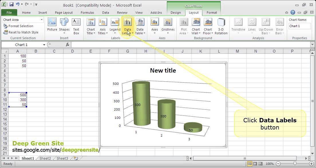
Change the format of data labels in a chart To get there, after adding your data labels, select the data label to format, and then click Chart Elements > Data Labels > More Options. To go to the appropriate area, click one of the four icons ( Fill & Line, Effects, Size & Properties ( Layout & Properties in Outlook or Word), or Label Options) shown here. Adding Data Labels to Your Chart (Microsoft Excel) To add data labels in Excel 2013 or Excel 2016, follow these steps: Activate the chart by clicking on it, if necessary. Make sure the Design tab of the ribbon is displayed. (This will appear when the chart is selected.) Click the Add Chart Element drop-down list. Select the Data Labels tool. Apply Custom Data Labels to Charted Points - Peltier Tech First, add labels to your series, then press Ctrl+1 (numeral one) to open the Format Data Labels task pane. I've shown the task pane below floating next to the chart, but it's usually docked off to the right edge of the Excel window.

Add data labels excel 2013. How to Print Labels from Excel - Lifewire Select Mailings > Write & Insert Fields > Update Labels . Once you have the Excel spreadsheet and the Word document set up, you can merge the information and print your labels. Click Finish & Merge in the Finish group on the Mailings tab. Click Edit Individual Documents to preview how your printed labels will appear. Select All > OK . How to Add Data Labels to your Excel Chart in Excel 2013 Watch this video to learn how to add data labels to your Excel 2013 chart. Data labels show the values next to the corresponding chart element, for instance a percentage... Format Data Labels in Excel- Instructions - TeachUcomp, Inc. To do this, click the "Format" tab within the "Chart Tools" contextual tab in the Ribbon. Then select the data labels to format from the "Chart Elements" drop-down in the "Current Selection" button group. Then click the "Format Selection" button that appears below the drop-down menu in the same area. mail.google.com › mailgoogle mail We would like to show you a description here but the site won’t allow us.

› add-vertical-line-excel-chartAdd vertical line to Excel chart: scatter plot, bar and line ... May 15, 2019 · In Excel 2013, Excel 2016, Excel 2019 and later, select Combo on the All Charts tab, choose Scatter with Straight Lines for the Average series, and click OK to close the dialog. In Excel 2010 and earlier, select X Y (Scatter) > Scatter with Straight Lines , and click OK . How to Data Labels in a Line Graph in Excel 2013 - YouTube Want to insert Data Labels in a line graph in Microsoft® Excel 2013? Follow the easy steps shown in this video. Content in this video is provided on an ""as ... Add or remove data labels in a chart - support.microsoft.com To label one data point, after clicking the series, click that data point. In the upper right corner, next to the chart, click Add Chart Element > Data Labels. To change the location, click the arrow, and choose an option. If you want to show your data label inside a text bubble shape, click Data Callout. How to Add Data Tables to Charts in Excel 2013 - dummies To add a data table to your selected chart and position and format it, click the Chart Elements button next to the chart and then select the Data Table check box before you select one of the following options on its continuation menu:

Add a DATA LABEL to ONE POINT on a chart in Excel All the data points will be highlighted. Click again on the single point that you want to add a data label to. Right-click and select ' Add data label '. This is the key step! Right-click again on the data point itself (not the label) and select ' Format data label '. You can now configure the label as required — select the content of ... How to Use Cell Values for Excel Chart Labels - How-To Geek Select the chart, choose the "Chart Elements" option, click the "Data Labels" arrow, and then "More Options.". Uncheck the "Value" box and check the "Value From Cells" box. Select cells C2:C6 to use for the data label range and then click the "OK" button. The values from these cells are now used for the chart data labels. Values From Cell: Missing Data Labels Option in Excel 2013? Insert data labels Edit each individual data label In the formula bar enter a formula that points to the cell that holds the desired label. This process can be tedious for larger charts with many labels. You can download and install the free XY Chart Labeler, which automates the process and still works fine with Excel 2103. Telling a story with charts in Excel 2013 - Microsoft 365 Blog Select the data labels by clicking on one. In the Task Pane, click the Label Options tab (the bar chart icon). Click the Label Options subheading to expand it. Uncheck the Category Name box. Then, to delete some individual data labels until only the high and low point labels are left, I can: Select all data labels by clicking on one.

Format Number Options for Chart Data Labels in Excel 2011 for Mac

How to Change Excel Chart Data Labels to Custom Values? First add data labels to the chart (Layout Ribbon > Data Labels) Define the new data label values in a bunch of cells, like this: Now, click on any data label. This will select "all" data labels. Now click once again. At this point excel will select only one data label. Go to Formula bar, press = and point to the cell where the data label ...

MS Excel 2010 / How to remove data labels from the chart - YouTube

How to Insert Axis Labels In An Excel Chart | Excelchat How to add vertical axis labels in Excel 2016/2013 We will again click on the chart to turn on the Chart Design tab We will go to Chart Design and select Add Chart Element Figure 6 - Insert axis labels in Excel In the drop-down menu, we will click on Axis Titles, and subsequently, select Primary vertical

31 What Is Data Label In Excel - Labels Database 2020

Excel charts: add title, customize chart axis, legend and data labels ... Click anywhere within your Excel chart, then click the Chart Elements button and check the Axis Titles box. If you want to display the title only for one axis, either horizontal or vertical, click the arrow next to Axis Titles and clear one of the boxes: Click the axis title box on the chart, and type the text.

35 What Is Data Label In Excel - Labels For You

How to Customize Chart Elements in Excel 2013 - dummies To add data labels to your selected chart and position them, click the Chart Elements button next to the chart and then select the Data Labels check box before you select one of the following options on its continuation menu: Center to position the data labels in the middle of each data point

Format Number Options for Chart Data Labels in Excel 2011 for Mac

› excel_barcodeExcel Barcode Generator Add-in: Create Barcodes in Excel 2019 ... Free Download. Create 30+ barcodes into Microsoft Office Excel Spreadsheet with this Barcode Generator for Excel Add-in. No Barcode Font, Excel Macro, VBA, ActiveX control to install. Completely integrate into Microsoft Office Excel 2019, 2016, 2013, 2010 and 2007; Easy to convert text to barcode image, without any VBA, barcode font, Excel ...

How to Make Labels from Excel

Quick Tip: Excel 2013 offers flexible data labels | TechRepublic right-click and choose Insert Data Label Field. In the next dialog, select [Cell] Choose Cell. When Excel displays the source dialog, click the cell that contains the MIN () function, and click OK....

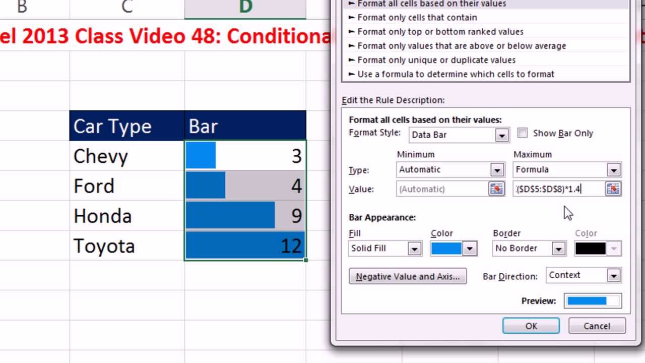
Highline Excel 2013 Class Video 48: Conditional Formatting: Bar Chart with Data Labels - YouTube

Custom Data Labels with Colors and Symbols in Excel Charts - [How To] Step 4: Select the data in column C and hit Ctrl+1 to invoke format cell dialogue box. From left click custom and have your cursor in the type field and follow these steps: Press and Hold ALT key on the keyboard and on the Numpad hit 3 and 0 keys. Let go the ALT key and you will see that upward arrow is inserted.

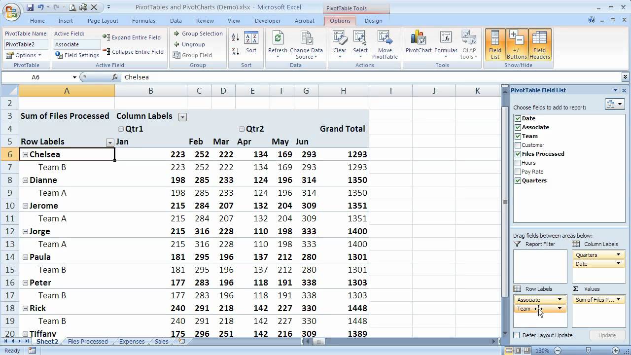
How to group row labels in Excel 2007 PivotTables (Excel 07-104) - YouTube

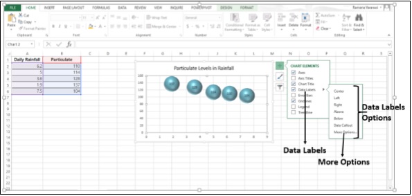
How to Add Data Labels in Excel - Excelchat | Excelchat How to Add Data Labels In Excel 2013 And Later Versions In Excel 2013 and the later versions we need to do the followings; Click anywhere in the chart area to display the Chart Elements button Figure 5. Chart Elements Button Click the Chart Elements button > Select the Data Labels, then click the Arrow to choose the data labels position. Figure 6.

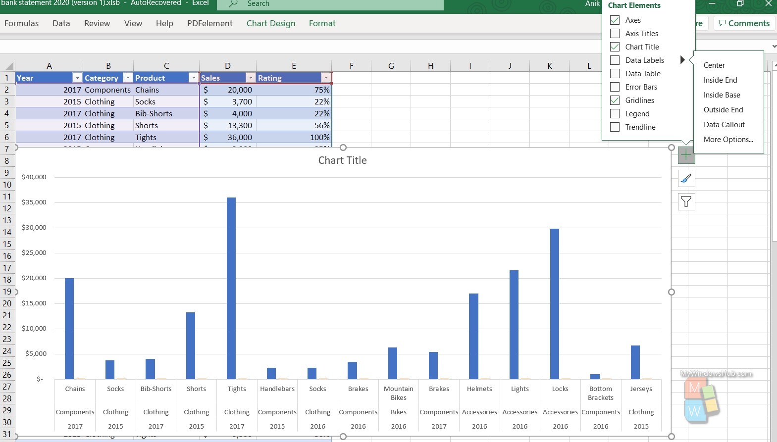
How To Show Or Hide Data Labels On MS Excel? | My Windows Hub

Creating a chart with dynamic labels - Microsoft Excel 2013 The trick of this chart is to show data from specific cells in the chart labels. For example, if you have to show in one chart two different data bar: To compare two different teams, you should create a chart using percent of task completing (in this example, cells C15:D15).

Ammo box labels « Ultimate Reloader Reloading Blog

How to add data labels from different column in an Excel chart? Right click the data series in the chart, and select Add Data Labels > Add Data Labels from the context menu to add data labels. 2. Click any data label to select all data labels, and then click the specified data label to select it only in the chart. 3.

How to Create Multi-Category Chart in Excel - Excel Board

Excel 2013 Bing Map App -- Customize Labels and Focus Excel 2013 Bing Map App -- Customize Labels and Focus. I'm testing the Bing Map app in Excel 2013. I see how the data can be easily plotted by location name, and values in the next column. What I'd like to know is: If you're plotting lat/longs as the location -- can you have a "name" associated with that to display for each point on the map ...

Example: Charts with Data Tools — XlsxWriter Documentation

Label Options for Chart Data Labels in PowerPoint 2013 for Windows In this Task Pane, make sure that the Label Options tab, as shown highlighted in red within Figure 1, below is selected. Then, click the Label Options button, as shown highlighted in blue within Figure 1. Figure 1: Label Options within Format Data Labels Task Pane. As you can see in Figure 1 above, Label Options have been divided into two ...

Two-Level Axis Labels (Microsoft Excel)

How to add or move data labels in Excel chart? - ExtendOffice To add or move data labels in a chart, you can do as below steps: In Excel 2013 or 2016. 1. Click the chart to show the Chart Elements button .. 2. Then click the Chart Elements, and check Data Labels, then you can click the arrow to choose an option about the data labels in the sub menu.See screenshot:

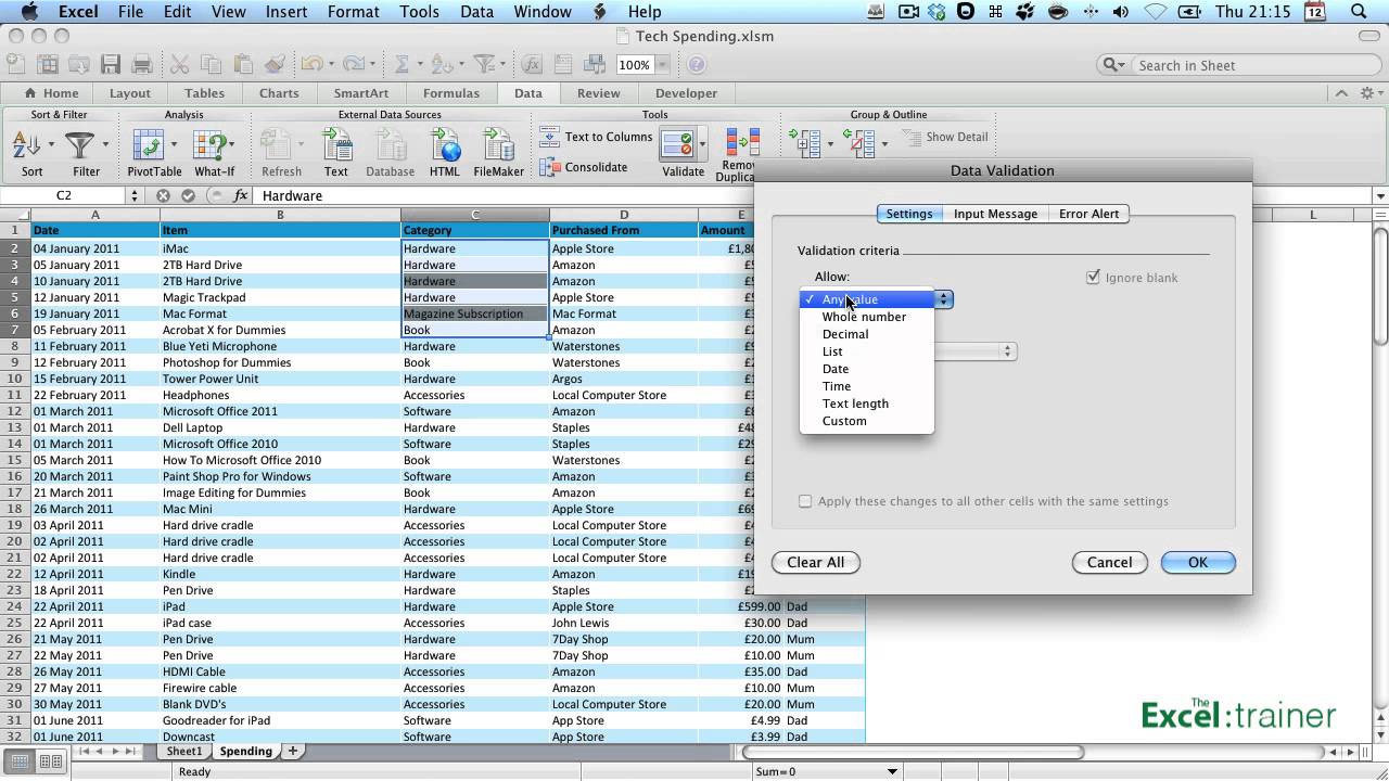
Excel : Data Validation & Drop Down Lists - YouTube

Adding rich data labels to charts in Excel 2013 - Microsoft 365 Blog To add a data label in a shape, select the data point of interest, then right-click it to pull up the context menu. Click Add Data Label, then click Add Data Callout . The result is that your data label will appear in a graphical callout. In this case, the category Thr for the particular data label is automatically added to the callout too.

Format Data Labels in Excel- Instructions | Microsoft excel, Microsoft, Bar chart

support.microsoft.com › en-us › officeUpdate the data in an existing chart - support.microsoft.com After you create a chart, you can edit the data in the Excel sheet. The changes will be reflected in the chart. Click the chart. Excel highlights the data table that is used for the chart. The gray fill indicates a row or column used for the category axis. The red fill indicates a row or column that contains data series labels.

Add or Remove Data Labels in excel - YouTube

Apply Custom Data Labels to Charted Points - Peltier Tech First, add labels to your series, then press Ctrl+1 (numeral one) to open the Format Data Labels task pane. I've shown the task pane below floating next to the chart, but it's usually docked off to the right edge of the Excel window.

Advanced Excel - более богатые метки данных - CoderLessons.com

Adding Data Labels to Your Chart (Microsoft Excel) To add data labels in Excel 2013 or Excel 2016, follow these steps: Activate the chart by clicking on it, if necessary. Make sure the Design tab of the ribbon is displayed. (This will appear when the chart is selected.) Click the Add Chart Element drop-down list. Select the Data Labels tool.

Share :