43 excel 2013 pie chart labels

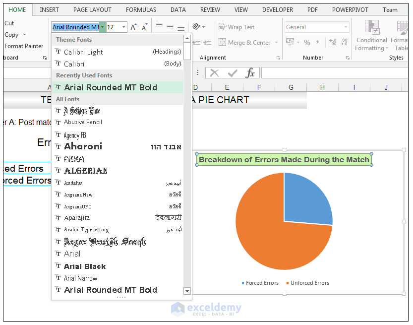
How to Create Exploding Pie Charts in Excel - Lifewire Right-click the current chart to open the context menu. In the menu, click Change Chart Type to open the Change Chart Type dialog box . In the dialog box, click the All Charts tab. Click Pie in the left side pane and then click Pie of Pie or Bar of Pie in the right pane for the dialog box. Changing the Number of Data Points Creating a pie chart and display whole numbers, not percentages. You don't want to change the format, you want to change the SOURCE of the data label. You want to right click on the pie chart so the pie is selected. Choose the option "Format Data Series...". Under the Tab "Data Labels" and Under Label Contains check off "Value". The number value from the source should now be your slice labels. g-

Excel 2013 Pie Chart Category Data Labels keep Disappearing GeneLandriau2 Created on April 19, 2016 Excel 2013 Pie Chart Category Data Labels keep Disappearing Hi All, I have a table in Excel 2013 with 2 slicers - Region and Product Hierarachy, with 5 values in each. I've built a couple pie charts that update when you click on the slicers, to show Market Share by Market Segment.

Excel 2013 pie chart labels

How to Make Charts and Graphs in Excel | Smartsheet Jan 22, 2018 · Use this step-by-step how-to and discover the easiest and fastest way to make a chart or graph in Excel. Learn when to use certain chart types and graphical elements. ... Each value is represented as a piece of the pie so you can identify the proportions. There are five pie chart types: pie, pie of pie (this breaks out one piece of the pie into ... Excel Gauge Chart Template - Free Download - How to Create Step #7: Add the pointer data into the equation by creating the pie chart. Step #8: Realign the two charts. Step #9: Align the pie chart with the doughnut chart. Step #10: Hide all the slices of the pie chart except the pointer and remove the chart … Excel Pie Chart Multiple Series - TheRescipes.info How to Create Pie Charts in Excel (In Easy Steps) great To create a pie chart of the 2017 data series, execute the following steps. 1. Select the range A1:D2. 2. On the Insert tab, in the Charts group, click the Pie symbol. 3. Click Pie. 4. Click on the pie to select the whole pie. See more result ›› 43 Visit site

Excel 2013 pie chart labels. Pie Charts in Power View - YouTube Pie charts are simple or sophisticated in Power View. This video shows you how to create a basic pie chart, add slices, and drill down and drill up.Olympics ... Excel 2013 Recommended Charts, Secondary Axis, Scatter & PivotCharts Excel 2013 includes a brilliant new option for creating charts called Recommended Charts. Recommended Charts is able to look at the nature of your data and present you with a choice of the most suitable chart types it thinks you should use. In other words it will recognise whether you data will be best displayed… Read More »Excel 2013 Recommended Charts, Secondary Axis, Scatter & PivotCharts How to Make a Pie Chart in Excel 2013 - Solve Your Tech How to Make Excel 2013 Pie Charts Open your spreadsheet. Select the data. Click the Insert tab. Select the Pie Chart button. Choose the desired pie chart style. Our article continues below with additional information on making a piechart in Excel, including pictures of these steps. How to Create a Pie Chart in Excel (Guide with Pictures) How to make a chart (graph) in Excel and save it as template Oct 22, 2015 · 3. Inset the chart in Excel worksheet. To add the graph on the current sheet, go to the Insert tab > Charts group, and click on a chart type you would like to create.. In Excel 2013 and Excel 2016, you can click the Recommended Charts button to view a gallery of pre-configured graphs that best match the selected data.. In this example, we are creating a 3-D …

Pie charts in Power View - support.microsoft.com Drag a category field to the Slices box. Create a drill-down pie chart Drag another category field to the Color box, under the field that's already in that box. The pie chart looks unchanged. Double-click one of the pie colors. The colors of the pie chart now show the percentages of the second field, filtered for the pie color you double-clicked. Add a pie chart - support.microsoft.com To switch to one of these pie charts, click the chart, and then on the Chart Tools Design tab, click Change Chart Type. When the Change Chart Type gallery opens, pick the one you want. See Also. Select data for a chart in Excel. Create a chart in Excel. Add a chart to your document in Word. Add a chart to your PowerPoint presentation Micro Center - Articles Get the facts you need to build your own computer, learn more about new technology, or find answers to questions. Browse our library of support and how-to articles, resources, and helpful hints on a wide range of computers and electronics. Display data point labels outside a pie chart in a paginated report ... Create a pie chart and display the data labels. Open the Properties pane. On the design surface, click on the pie itself to display the Category properties in the Properties pane. Expand the CustomAttributes node. A list of attributes for the pie chart is displayed. Set the PieLabelStyle property to Outside. Set the PieLineColor property to Black.

Rotate a pie chart - support.microsoft.com If you want to rotate another type of chart, such as a bar or column chart, you simply change the chart type to the style that you want. For example, to rotate a column chart, you would change it to a bar chart. Select the chart, click the Chart Tools Design tab, and then click Change Chart Type. See Also. Add a pie chart. Available chart types ... How to Create a Waterfall Chart in Excel – Automate Excel This tutorial will demonstrate how to create a waterfall chart in all versions of Excel: 2007, 2010, 2013, 2016, and 2019. Waterfall Chart – Free Template Download Download our free Waterfall Chart Template for Excel. Download Now A waterfall chart (also called a bridge chart, flying bricks chart, cascade chart, or Mario chart) is a… Group Smaller Slices in Pie Charts to Improve Readability Select "Pie of Pie" chart, the one that looks like this: At this point the chart should look something like this: 2. Click on any slice and go to "format series". Click on any slice and hit CTRL+1 or right click and select format option. In the resulting dialog, you can change the way excel splits 2 pies. We will ask excel to split the ... How to modify Chart legends in Excel 2013 - Stack Overflow The words in the legend are sourced from the series name. You can point the series name to any cell in the spreadsheet. In the screenshot, the original series names were one, two and three. In the series definition, they got re-pointed to the cells that say blue, red and green. Depending on your data and requirements this can be made dynamic. Share

How to Make a Pie Chart in Excel & Add Rich Data Labels to The Chart!

Steps to Create Map Chart in Excel with Examples - EDUCBA Step 9: Click on the navigation down arrow available besides the Chart Options.It will open up several chart options. Click on Chart Title and add the title as “Country-Wise Sales” for this chart.Also, select the last option available, namely Series “Sales Amount”.This allows you to make customized changes into series data (numeric values in this case).

How to Create and Label a Pie Chart in Excel 2013 : 8 Steps - Instructables

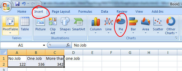
How to Make a Pie Chart in Excel - Contextures Blog Insert the Chart. After your data is set up, follow these steps to insert a pie chart: Select any cell in the data. On the Excel Ribbon, click the Insert tab. In the Charts group, click Pie. Then, click the first pie option, at the top left. Do not be lured by any of the other options, like exploded pie, or worst of all, a 3-D pie.

Excel 3-D Pie charts - Microsoft Excel 2013

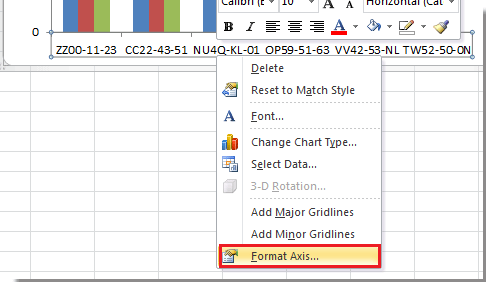
Excel 2013 Chart label not displaying The pie chart displays the wedge within the chart itself, but does not display the label. At the moment I have data labels with percentages. All other labels display, of which there are 7. I found a solution that fixes the problem each time it arises and that is to select Chart Tools/Format/Series 1 data labels and then Format Selection.

How to Create Multi-Category Chart in Excel - Excel Board

How to create waterfall chart in Excel 2016, 2013, 2010 - Ablebits Jul 25, 2014 · A waterfall chart is also known as an Excel bridge chart since the floating columns make a so-called bridge connecting the endpoints. These charts are quite useful for analytical purposes. If you need to evaluate a company profit or product earnings, make an inventory or sales analysis or just show how the number of your Facebook friends ...

How to Create A Pie Chart in Excel – Better Tech Tips

How To Add and Remove Legends In Excel Chart? - EDUCBA This has been a guide to Legend in Chart. Here we discuss how to add, remove and change the position of legends in an Excel chart, along with practical examples and a downloadable excel template. You can also go through our other suggested articles – Line Chart in Excel; Excel Bar Chart; Pie Chart in Excel; Scatter Chart in Excel

How to Create and Label a Pie Chart in Excel 2013 : 8 Steps - Instructables

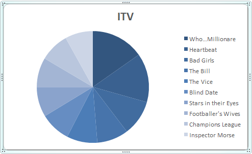
Legend Entry Tricks in Excel Charts - Peltier Tech In a pie chart, the legend labels are the category labels The easiest and most reliable way to set up data for a chart is to put category labels (or X values) in a column and (Y) values in the next column, then put a label in the cell above every value column (a pie chart has one value column) and leave the cell above the category labels blank.

Microsoft Excel Tutorials: How to Create a Pie Chart

How to create pie of pie or bar of pie chart in Excel? The following steps can help you to create a pie of pie or bar of pie chart: 1. Create the data that you want to use as follows: 2. Then select the data range, in this example, highlight cell A2:B9. And then click Insert > Pie > Pie of Pie or Bar of Pie, see screenshot: 3. And you will get the following chart: 4.

How to Adjust Pie Chart Labels in Excel : MS Excel Tips - YouTube

How to Add and Format Text Boxes in a Chart in Excel 2013 Excel 2013 For Dummies. To add a text box in Excel 2013 like the one shown to the chart when a chart is selected, select the Format tab under the Chart Tools contextual tab. Then, click the Insert Shapes drop-down button to open its palette where you select the Text Box button. To insert a text box in a worksheet when a chart or some other type ...

Excel 2007 - Create Custom Pie Chart (For Example With Horizontal Data) | The Solaris Cookbook ...

Rotate a pie chart - support.microsoft.com Right-click any slice of the pie chart > Format Data Series. In the Format Data Point pane in the Angle of first slice box, replace 0 with 120 and press Enter. Now, the pie chart looks like this: If you want to rotate another type of chart, such as a bar or column chart, you simply change the chart type to the style that you want.

Excel Professor: Speedometer Chart / Gas Gauge Chart

Excel Chart VBA - 33 Examples For Mastering Charts in Excel VBA 13. Example to set the type as a Pie Chart in Excel VBA. The following VBA code using xlPie constant to plot the Pie chart. Please check here for list of enumerations available in Excel VBA Charting. Sub Ex_ChartType_Pie_Chart() Dim cht As Object Set cht = ActiveSheet.ChartObjects.Add(Left:=300, Width:=300, Top:=10, Height:=300) With cht

32 How To Label A Pie Chart In Excel - Labels Information List

Broken Y Axis in an Excel Chart - Peltier Tech Nov 18, 2011 · The primary axis then bisects the chart and the secondary is at the bottom of the chart. I usually hide the labels and often the tick marks for the primary axis. ... then select Up/Down Bars from the Plus icon next to the chart in Excel 2013 or the Chart Tools > Layout tab in 2007/2010. ... She also criticised 3D charts, bar charts without a ...

How to rotate axis labels in chart in Excel?

How to Create Charts From the Ribbon in Excel 2013 - dummies Insert Pie or Doughnut Chart to preview your data as a 2-D or 3-D pie chart or 2-D doughnut chart Insert Scatter (X,Y) or Bubble Chart to preview your data as a 2-D scatter (X,Y) or bubble chart When using the galleries attached to these chart command buttons on the Insert tab to preview your data as a particular chart style, you can embed the ...

How to add titles to charts in Excel 2010 / 2013 in a minute.

How to Create and Label a Pie Chart in Excel 2013 Open Microsoft Excel 2013 and click on the "Blank workbook" option. Add Tip Ask Question Comment Download Step 2: Input the Data Create your spreadsheet by inputting the numbers and labels which are going to be used in the pie chart. In this example, I used the labels "Desserts", "Appertizers", "Entrees", "Beer", and "Wine". Add Tip Ask Question

How to Make a Pie Chart in Excel 2013 - Solve Your Tech

Excel 2010 Chart autofit option greyed out. I was able to resize in Excel 2016 by removing the axis labels, resizing the chart, and adding the labels back in. Right Click on the axis title and select Labels, Label Position = NONE. Resize your chart. Once resized add the axis title back on (from Axis Options change the label position back to Next to Axis).

Stats - Pie Charts

How to Create Pie Charts in Excel (In Easy Steps) Click the + button on the right side of the chart and click the check box next to Data Labels. 10. Click the paintbrush icon on the right side of the chart and change the color scheme of the pie chart. Result: 11. Right click the pie chart and click Format Data Labels. 12. Check Category Name, uncheck Value, check Percentage and click Center.

Excel 2010 pie chart data labels in case of "Best Fit"

How to hide datapoint label when value is zero in pie chart in report viwer Hi, I am using Repor viwer conrol in vs 2010. I have put pie char on report viwer. I want to hide datapoint label when value is zero. Please help me.

How to add titles to charts in Excel 2016 - 2010 in a minute.

Pie Chart Rounding in Excel - Peltier Tech Both charts below use the same data range, three cells each containing the value 1. Each pie wedge is 1/3 of the total, 33.333333…%, rounded to 33%. However, the first chart reports percentages of 34%, 33%, and 33%. The second chart, with one added decimal digit of precision, correctly displays 33.3% for all three wedges.

How to Add an Axis Title to an Excel Chart | Techwalla

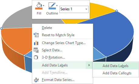
Microsoft Excel Tutorials: Add Data Labels to a Pie Chart To add the numbers from our E column (the viewing figures), left click on the pie chart itself to select it: The chart is selected when you can see all those blue circles surrounding it. Now right click the chart. You should get the following menu: From the menu, select Add Data Labels. New data labels will then appear on your chart:

Share :