45 change data labels in excel chart
c# - How do I change a data label on an excel bar chart to inside base ... I'm trying to change the position of the data label to Inside Base, but when I look inside the ExcelBarChart object I see an ExcelChartDataLabel property, and inside that a property named eLabelPosition. eLabelPosition is protected however and inaccessible. What is the proper way to set the data label position using EPPlus? Add a DATA LABEL to ONE POINT on a chart in Excel Click on the chart line to add the data point to. All the data points will be highlighted. Click again on the single point that you want to add a data label to. Right-click and select ' Add data label ' This is the key step! Right-click again on the data point itself (not the label) and select ' Format data label '.
Adding Data Labels to a Chart Using VBA Loops - Wise Owl One way to do this is by manually adding data labels to the chart within Excel, but we're going to achieve the same result in a single line of code. To do this, add the following line to your code: 'make sure data labels are turned on FilmDataSeries.HasDataLabels = True

Change data labels in excel chart
How to add or move data labels in Excel chart? - ExtendOffice In Excel 2013 or 2016. 1. Click the chart to show the Chart Elements button . 2. Then click the Chart Elements, and check Data Labels, then you can click the arrow to choose an option about the data labels in the sub menu. See screenshot: In Excel 2010 or 2007. 1. click on the chart to show the Layout tab in the Chart Tools group. See ... Excel charts: add title, customize chart axis, legend and data labels ... Adding data labels to Excel charts. To make your Excel graph easier to understand, you can add data labels to display details about the data series. ... Data label tips: To change the position of a given data label, click it and drag to where you want using the mouse. To change the labels' font and background color, select them, ... excel - Change format of all data labels of a single series at once ... Go to the chart and left mouse click on the 'data series' you want to edit. Click anywhere in formula bar above. Don't change anything. Click the 'tick icon' just to the left of the formula bar. Go straight back to the same data series and right mouse click, and choose add data labels This has worked in Excel 2016.
Change data labels in excel chart. How to format axis labels as thousands/millions in Excel? Right click at the axis you want to format its labels as thousands/millions, select Format Axisin the context menu. 2. In the Format Axisdialog/pane, click Number tab, then in theCategorylist box, select Custom, and type[>999999] #,,"M";#,"K"into Format Codetext box, and click Addbutton to add it toTypelist. See screenshot: 3. How to rotate axis labels in chart in Excel? - ExtendOffice Go to the chart and right click its axis labels you will rotate, and select the Format Axis from the context menu. 2. In the Format Axis pane in the right, click the Size & Properties button, click the Text direction box, and specify one direction from the drop down list. See screen shot below: The Best Office Productivity Tools How to add data labels from different column in an Excel chart? Right click the data series in the chart, and select Add Data Labels > Add Data Labels from the context menu to add data labels. 2. Click any data label to select all data labels, and then click the specified data label to select it only in the chart. 3. How to I rotate data labels on a column chart so that they are ... To change the text direction, first of all, please double click on the data label and make sure the data are selected (with a box surrounded like following image). Then on your right panel, the Format Data Labels panel should be opened. Go to Text Options > Text Box > Text direction > Rotate
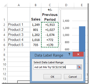
How to Rename a Data Series in Microsoft Excel To do this, right-click your graph or chart and click the "Select Data" option. This will open the "Select Data Source" options window. Your multiple data series will be listed under the "Legend Entries (Series)" column. To begin renaming your data series, select one from the list and then click the "Edit" button. Edit titles or data labels in a chart - support.microsoft.com The first click selects the data labels for the whole data series, and the second click selects the individual data label. Right-click the data label, and then click Format Data Label or Format Data Labels. Click Label Options if it's not selected, and then select the Reset Label Text check box. Top of Page How to Change Excel Chart Data Labels to Custom Values? You can change data labels and point them to different cells using this little trick. First add data labels to the chart (Layout Ribbon > Data Labels) Define the new data label values in a bunch of cells, like this: Now, click on any data label. This will select "all" data labels. Now click once again. Column Chart That Displays Percentage Change or Variance - Excel Campus Select the chart, go to the Format tab in the ribbon, and select Series "Invisible Bar" from the drop-down on the left side. Choose Data Labels > More Options from the Elements menu. Select the Label Options sub menu in the Format Data Labels task pane. Click the Value from Cells checkbox.
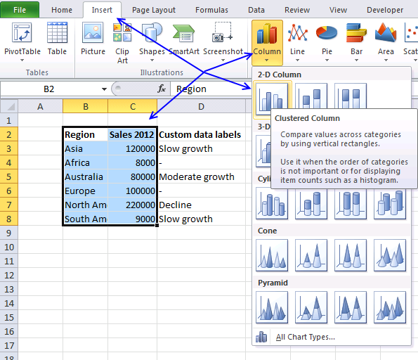
Add or remove data labels in a chart - support.microsoft.com Click the data series or chart. To label one data point, after clicking the series, click that data point. In the upper right corner, next to the chart, click Add Chart Element > Data Labels. To change the location, click the arrow, and choose an option. If you want to show your data label inside a text bubble shape, click Data Callout. Excel Chart Data Labels-Modifying Orientation - Microsoft Community You can right click on the data label part then select Format Axis. Click on the Size & Properties tab then adjust the Text Direction or Custom Angle. Thanks, Mike Report abuse 6 people found this reply helpful · Was this reply helpful? Yes No Change axis labels in a chart - support.microsoft.com Right-click the category labels you want to change, and click Select Data. In the Horizontal (Category) Axis Labels box, click Edit. In the Axis label range box, enter the labels you want to use, separated by commas. For example, type Quarter 1,Quarter 2,Quarter 3,Quarter 4. Change the format of text and numbers in labels How to show percentages in stacked column chart in Excel? Add percentages in stacked column chart 1. Select data range you need and click Insert > Column > Stacked Column. See screenshot: 2. Click at the column and then click Design > Switch Row/Column. 3. In Excel 2007, click Layout > Data Labels > Center . In Excel 2013 or the new version, click Design > Add Chart Element > Data Labels > Center. 4.
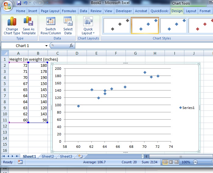
Scatter Plot / Scatter Chart: Definition, Examples, Excel/TI-83/TI-89/SPSS - Statistics How To
How to Get Colors in Excel Chart Data Lables - Formatting Trick How you can get colors in Axis Labels. First apply data labels to your chart and now select the data labels and press ctrl+1 (aww, come on now, you are reading this blog, you should what ctrl+1 means) and go to numbers tab. Select "custom" as category and specify the formatting code like this:

Quickly Create A Variable Width Column Chart In Excel
Move data labels - support.microsoft.com Click any data label once to select all of them, or double-click a specific data label you want to move. Right-click the selection > Chart Elements > Data Labels arrow, and select the placement option you want. Different options are available for different chart types.

Chapter 3 Excel 2007/2010 Charts
How to create Custom Data Labels in Excel Charts Create the chart as usual. Add default data labels. Click on each unwanted label (using slow double click) and delete it. Select each item where you want the custom label one at a time. Press F2 to move focus to the Formula editing box. Type the equal to sign. Now click on the cell which contains the appropriate label.

How to Add Data Labels in Excel - Excelchat | Excelchat
How to Customize Your Excel Pivot Chart Data Labels - dummies To add data labels, just select the command that corresponds to the location you want. To remove the labels, select the None command. If you want to specify what Excel should use for the data label, choose the More Data Labels Options command from the Data Labels menu. Excel displays the Format Data Labels pane.
How-to Use Data Labels from a Range in an Excel Chart - Excel Dashboard Templates
Add / Move Data Labels in Charts - Excel & Google Sheets Adding Data Labels Click on the graph Select + Sign in the top right of the graph Check Data Labels Change Position of Data Labels Click on the arrow next to Data Labels to change the position of where the labels are in relation to the bar chart Final Graph with Data Labels
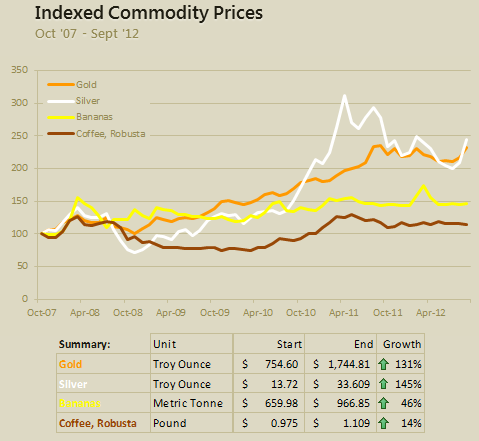
What is an indexed chart and how to create one using Excel?
Change the format of data labels in a chart To get there, after adding your data labels, select the data label to format, and then click Chart Elements > Data Labels > More Options. To go to the appropriate area, click one of the four icons ( Fill & Line, Effects, Size & Properties ( Layout & Properties in Outlook or Word), or Label Options) shown here.

410 How to display percentage labels in pie chart in Excel 2016 - YouTube
Change the labels in an Excel data series | TechRepublic Click the Chart Wizard button in the Standard toolbar. Click Next. Click the Series tab. Click the Window Shade button in the Category (X) Axis. Labels box. Select B3:D3 to select the labels in ...

How to Change Excel Chart Data Labels to Custom Values? | Chandoo.org - Learn Microsoft Excel Online
Custom Data Labels with Colors and Symbols in Excel Charts - [How To] Step 4: Select the data in column C and hit Ctrl+1 to invoke format cell dialogue box. From left click custom and have your cursor in the type field and follow these steps: Press and Hold ALT key on the keyboard and on the Numpad hit 3 and 0 keys. Let go the ALT key and you will see that upward arrow is inserted.
Data labels on Excel charts « projectwoman.com
How to Use Cell Values for Excel Chart Labels Select the chart, choose the "Chart Elements" option, click the "Data Labels" arrow, and then "More Options.". Uncheck the "Value" box and check the "Value From Cells" box. Select cells C2:C6 to use for the data label range and then click the "OK" button. The values from these cells are now used for the chart data labels.

Enable or Disable Excel Data Labels at the click of a button - How To - PakAccountants.com
excel - Change format of all data labels of a single series at once ... Go to the chart and left mouse click on the 'data series' you want to edit. Click anywhere in formula bar above. Don't change anything. Click the 'tick icon' just to the left of the formula bar. Go straight back to the same data series and right mouse click, and choose add data labels This has worked in Excel 2016.

Date Axis in Excel Chart is wrong • AuditExcel.co.za
Excel charts: add title, customize chart axis, legend and data labels ... Adding data labels to Excel charts. To make your Excel graph easier to understand, you can add data labels to display details about the data series. ... Data label tips: To change the position of a given data label, click it and drag to where you want using the mouse. To change the labels' font and background color, select them, ...
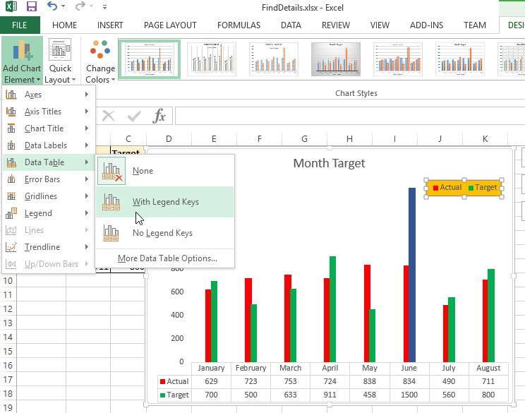
Chart axes, legend, data labels, trendline in Excel - Tech Funda
How to add or move data labels in Excel chart? - ExtendOffice In Excel 2013 or 2016. 1. Click the chart to show the Chart Elements button . 2. Then click the Chart Elements, and check Data Labels, then you can click the arrow to choose an option about the data labels in the sub menu. See screenshot: In Excel 2010 or 2007. 1. click on the chart to show the Layout tab in the Chart Tools group. See ...
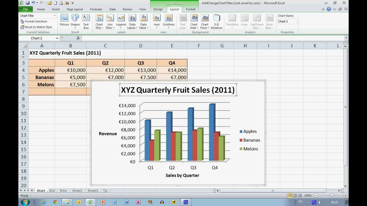
How To... Add and Change Chart Titles in Excel 2010 - YouTube

Excel Treemap - Beat Excel!

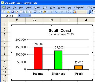
How to Make Excel Charts More Intuitive by Adding Data Labels and Tables - Data Recovery Blog

How to Add Data Labels in Excel - Excelchat | Excelchat
Custom data labels in a chart | Get Digital Help - Microsoft Excel resource

How-to Use Data Labels from a Range in an Excel Chart - Excel Dashboard Templates
Post a Comment for "45 change data labels in excel chart"